Numerical computation
Installation
On Julia's package mode, run the following commands.
pkg> add IntervalSets
pkg> add StaticArrays
pkg> add BasicBSpline
pkg> add BasicBSplineExporter.jl
pkg> add ElasticSurfaceEmbedding.jl
Overview of our method
Our theoretical framework is based on:
- Mathematical model: Nonlinear elasticity on Riemannian manifold
- Geometric representation: B-spline manifold
- Numerical analysis: Galerkin method, Newton-Raphson method
The computation process proceeds as shown in the following flowchart (from our paper):
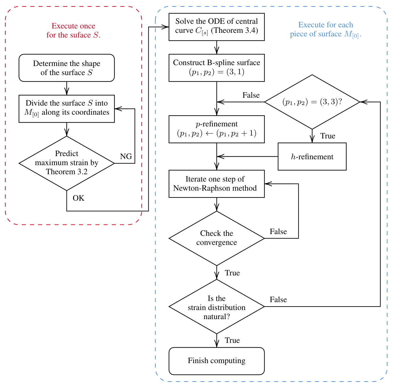
For more information, read our paper or contact me!
Example: Paraboloid
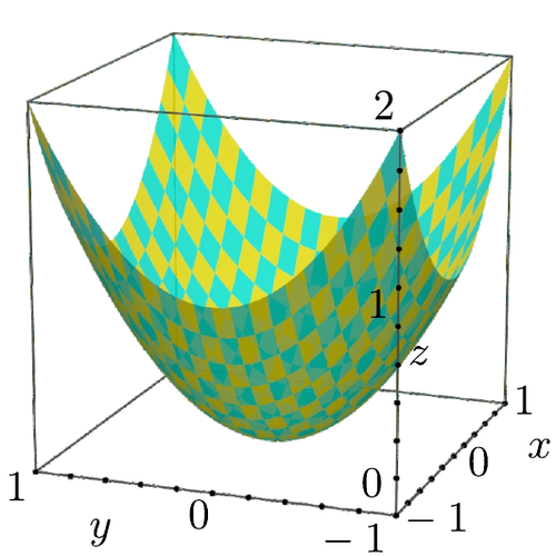
Through this section, we treat a paraboloid $z=x^2+y^2$ as an example.
Load packages, and optional configuration
Load packages with the following script.
using IntervalSets
using BasicBSpline
using StaticArrays
using ElasticSurfaceEmbedding
Define the shape of surface
ElasticSurfaceEmbedding.𝒑₍₀₎(u¹,u²) = SVector(u¹, u², u¹^2+u²^2)\[\begin{aligned} \bm{p}_{[0]}(u^1, u^2) &= \begin{pmatrix} u^1 \\ u^2 \\ (u^1)^2 + (u^2)^2 \end{pmatrix} \\ D &= [-1,1]\times[-1,1] \end{aligned}\]
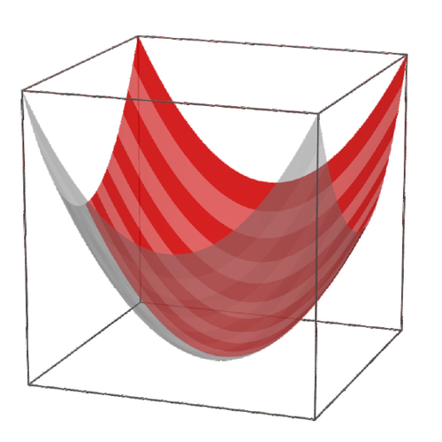
In the next step, we will split the surface into elongated strips. The domain of each strip should be rectangular, and the longer direction is u¹, and the shorter direction is u². The paraboloid has four‐fold symmetry, so we don't have to take care of it.
Split the surface into strips
The domain $D$ will be split into $D_i$.
\[\begin{aligned} D_i &= [-1,1]\times\left[\frac{i-1}{10},\frac{i}{10}\right] & (i=1,\dots,10) \end{aligned}\]
In julia script, just define a domain of the strip with function D(i,n).
n = 10
D(i,n) = (-1.0..1.0, (i-1)/n..i/n)
D (generic function with 1 method)Check the strain prediction
Before computing the embedding numerically, we can predict the strain with Strain Approximation Formula:
\[\begin{aligned} E_{11}^{\langle 0\rangle}&\approx\frac{1}{2}K_{[0]}B^2\left(r^2-\frac{1}{3}\right) \end{aligned}\]
You can check this strain estimation using the show_strain function.
for i in 1:n
    show_strain(D(i,n))
end
┌ Info: Strain - domain: [-1.0, 1.0]×[0.0, 0.1]
└ Predicted: (min: -0.001650165016501651, max: 0.0033003300330033025)
┌ Info: Strain - domain: [-1.0, 1.0]×[0.1, 0.2]
└ Predicted: (min: -0.0015290519877675841, max: 0.003058103975535171)
┌ Info: Strain - domain: [-1.0, 1.0]×[0.2, 0.3]
└ Predicted: (min: -0.0013333333333333326, max: 0.0026666666666666657)
┌ Info: Strain - domain: [-1.0, 1.0]×[0.3, 0.4]
└ Predicted: (min: -0.001118568232662193, max: 0.0022371364653243895)
┌ Info: Strain - domain: [-1.0, 1.0]×[0.4, 0.5]
└ Predicted: (min: -0.0009208103130755056, max: 0.0018416206261510117)
┌ Info: Strain - domain: [-1.0, 1.0]×[0.5, 0.6]
└ Predicted: (min: -0.000754147812971342, max: 0.0015082956259426892)
┌ Info: Strain - domain: [-1.0, 1.0]×[0.6, 0.7]
└ Predicted: (min: -0.0006195786864931844, max: 0.0012391573729863732)
┌ Info: Strain - domain: [-1.0, 1.0]×[0.7, 0.8]
└ Predicted: (min: -0.0005128205128205139, max: 0.001025641025641028)
┌ Info: Strain - domain: [-1.0, 1.0]×[0.8, 0.9]
└ Predicted: (min: -0.0004284490145672663, max: 0.0008568980291345356)
┌ Info: Strain - domain: [-1.0, 1.0]×[0.9, 1.0]
└ Predicted: (min: -0.00036153289949385377, max: 0.0007230657989877101)Positive number means tension, and negative number means compression. Empirically, it is better if the absolute value of strain is smaller than $0.01 (=1\%)$.
Initial state
If you finished checking the strain prediction, the next step is determination of the initial state with initial_state (or initial_state! from the second time).
From this section, the computing is done for each piece of the surface. First, let's calculate for $i=1$.
i = 11As a first step, let's compute the initial state.
steptree = initial_state(D(i,n))
Newton-Raphson method iteration
newton_onestep! function calculates one step of Newton-Raphson method iteration.
newton_onestep!(steptree, fixingmethod=:fix3points)
newton_onestep!(steptree)
You can choose the fixing method from below:
:default(default):fix3points
Refinement of B-spline manifold
refinement!(steptree, p₊=(0,1), k₊=(EmptyKnotVector(),KnotVector([(i-1/2)/10])))
The knotvector to be inserted in refinement! can be suggested by show_knotvector function.
Pin the step
If you finished computing for the strip, it's time to pin the step. This pin! function will be used for the the final export step.
pin!(steptree)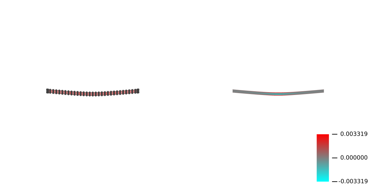
If you add a pin mistakenly, you can remove the pin with unpin! function.
unpin!(steptree, 4)
Compute more
newton_onestep!(steptree)
newton_onestep!(steptree)
pin!(steptree)

i = 2
initial_state!(steptree, D(i,n))
newton_onestep!(steptree, fixingmethod=:fix3points)
newton_onestep!(steptree)
refinement!(steptree, p₊=(0,1), k₊=(EmptyKnotVector(),KnotVector([(i-1/2)/10])))
newton_onestep!(steptree)
newton_onestep!(steptree)
pin!(steptree)
Export all pinned shapes
This is the final step of the computational process with export_pinned_steps.
export_pinned_steps(".", steptree, unitlength=(50, "mm"), mesh=(20,1), xlims=(-2,2), ylims=(-0.3,0.3))2-element Vector{String}:
"./pinned/pinned-6.svg"
"./pinned/pinned-12.svg"This will create SVG files in ./pinned.
pinned/pinned-6.svg 
pinned/pinned-12.svg 
The all outputs for i in 1:10 will be like this: 
You can edit these files, and craft them into curved surface shape.
Other examples
can be found in gallery