Knot vector

Setup

using BasicBSpline
using Plots

Definition

There are four sutypes of AbstractKnotVector; KnotVector, UniformKnotVector, SubKnotVector, and EmptyKnotVector.

julia> subtypes(AbstractKnotVector)4-element Vector{Any}:
 EmptyKnotVector{T} where T<:Real
 KnotVector{T} where T<:Real
 SubKnotVector{T, S} where {T<:Real, S<:(SubArray{T, 1})}
 UniformKnotVector{T} where T<:Real

They can be constructed like this.

julia> KnotVector([1,2,3])  # `KnotVector` stores a vector with `Vector{<:Real}`KnotVector([1, 2, 3])
julia> KnotVector(1:3)KnotVector([1, 2, 3])
julia> UniformKnotVector(1:8)  # `UniformKnotVector` stores a vector with `<:AbstractRange`UniformKnotVector(1:8)
julia> UniformKnotVector(8:-1:3)UniformKnotVector(3:1:8)
julia> view(KnotVector([1,2,3]), 2:3)  # Efficient and lazy knot vector with `view`SubKnotVector([2, 3])
julia> EmptyKnotVector()  # Sometimes `EmptyKnotVector` is useful.EmptyKnotVector{Bool}()
julia> EmptyKnotVector{Float64}()EmptyKnotVector{Float64}()

There is a useful string macro @knotvector_str that generates a KnotVector instance.

julia> knotvector"1231123"KnotVector([1, 2, 2, 3, 3, 3, 4, 5, 6, 6, 7, 7, 7])

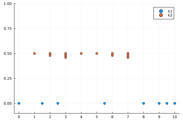
A knot vector can be visualized with Plots.plot.

julia> k1 = KnotVector([0.0, 1.5, 2.5, 5.5, 8.0, 9.0, 9.5, 10.0])KnotVector([0.0, 1.5, 2.5, 5.5, 8.0, 9.0, 9.5, 10.0])
julia> k2 = knotvector"1231123"KnotVector([1, 2, 2, 3, 3, 3, 4, 5, 6, 6, 7, 7, 7])
julia> gr()Plots.GRBackend()
julia> plot(k1; label="k1")Plot{Plots.GRBackend() n=1}
julia> plot!(k2; label="k2", offset=0.5, ylims=(-0.1,1), xticks=0:10)Plot{Plots.GRBackend() n=2}

Operations for knot vectors

Setup and visualization

k1 = knotvector"1 2 1 11 2 31"
k2 = knotvector"113 1 12 2 32 1  1"
plot(k1; offset=-0.0, label="k1", xticks=1:18, yticks=nothing, legend=:right)
plot!(k2; offset=-0.2, label="k2")
plot!(k1+k2; offset=-0.4, label="k1+k2")
plot!(2k1; offset=-0.6, label="2k1")
plot!(unique(k1); offset=-0.8, label="unique(k1)")
plot!(unique(k2); offset=-1.0, label="unique(k2)")
plot!(unique(k1+k2); offset=-1.2, label="unique(k1+k2)")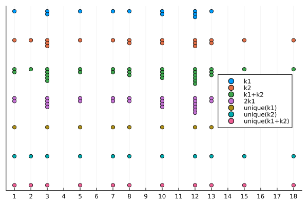

Length of a knot vector

length(k::AbstractKnotVector)

julia> length(k1)12
julia> length(k2)18

Addition of knot vectors

Although a knot vector is not a vector in linear algebra, but we introduce additional operator $+$.

Base.:+(k1::KnotVector{T}, k2::KnotVector{T}) where T

julia> k1 + k2KnotVector([1, 1, 2, 3, 3, 3, 3, 3, 5, 5, 7, 7, 8, 8, 8, 10, 10, 10, 10, 12, 12, 12, 12, 12, 12, 13, 13, 13, 15, 18])

Note that the operator +(::KnotVector, ::KnotVector) is commutative. This is why we choose the $+$ sign. We also introduce product operator $\cdot$ for knot vector.

Multiplication of knot vectors

*(m::Integer, k::AbstractKnotVector)

julia> 2*k1KnotVector([1, 1, 3, 3, 3, 3, 5, 5, 7, 7, 8, 8, 10, 10, 10, 10, 12, 12, 12, 12, 12, 12, 13, 13])
julia> 2*k2KnotVector([1, 1, 2, 2, 3, 3, 3, 3, 3, 3, 5, 5, 7, 7, 8, 8, 8, 8, 10, 10, 10, 10, 12, 12, 12, 12, 12, 12, 13, 13, 13, 13, 15, 15, 18, 18])

Generate a knot vector with unique elements

unique(k::AbstractKnotVector)

julia> unique(k1)KnotVector([1, 3, 5, 7, 8, 10, 12, 13])
julia> unique(k2)KnotVector([1, 2, 3, 5, 7, 8, 10, 12, 13, 15, 18])

Inclusive relationship between knot vectors

Base.issubset(k::KnotVector, k′::KnotVector)

julia> unique(k1) ⊆ k1 ⊆ k2true
julia> k1 ⊆ k1true
julia> k2 ⊆ k1false

Count knots in a knot vector

countknots(k::AbstractKnotVector, t::Real)

julia> countknots(k1, 0.5)0
julia> countknots(k1, 1.0)1
julia> countknots(k1, 3.0)2